
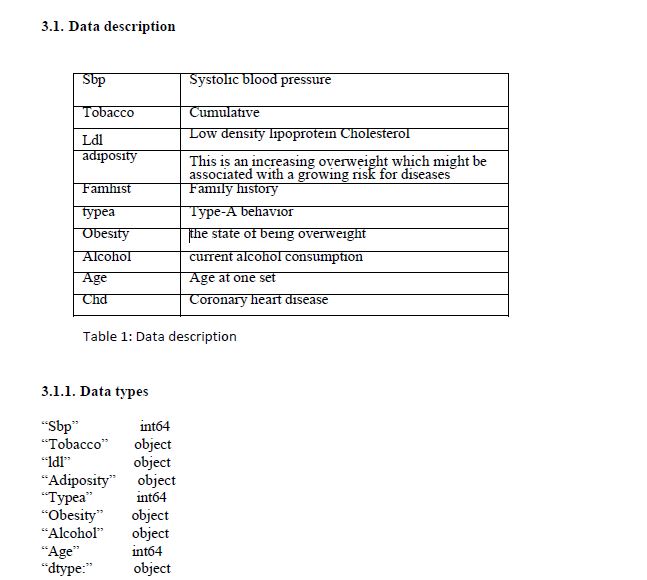
1. Introduction
Heart related disease remains amongst the major cause of death throughout the work from the past decade [1]. Cholesterol level, high blood pressure and diabetics are amongst the main contributing factors related to heart diseases. Amongst the risk factors associated with heart diseases can be traced back to family medical history, smoking and drinking patterns of a patient and port health diet. [2] data mining assist in the extraction of patterns that are found in the process of
knowledge discovery within the databases in which intelligent methodologies are applied. The emerging discoveries within the data mining domain that promise to provide intelligent tolls and new technologies which will assist the human to do analytics and gain understanding huge volumes of data remains a challenge with
unsolved problems. The current functions within data mining domain includes classifications, clustering, regression, and the discovery of association rules, rule generation, summarization, sequence analysis and dependency modelling. Numerous data mining challenges can be addressed effectively though the use of soft computing techniques. Amongst this technique are neural network, generic algorithms, fuzzy logic that will ultimately leads an intelligent very interpretable and
solutions that are low cost compared to traditional techniques. Dimension reduction is regarded amongst the mostly used method for data mining for the extraction of patterns in a more reliable and intelligent manner and has widely been used to find models that
data relationships [3]. The rest of the paper is organized as follows. In Section 2, some background on dimensionality Reduction Algorithms are discussed. In Section 3, the methodology and the simulation results obtained are presented. Finally, Section 4 concludes the paper.
2. Background
The dimensionality reduction can be regarded as an unsupervised learning technique, which may be applied as pre-processing step for data transformation towards machine learning algorithms on both regression predictive modelling and classification datasets with supervised learning algorithms. Furthermore, dimensionality reduction represents a technique which may be adopted for dropping the amount of input variables in training data. Every time one is dealing with a large capacity of dimensional data, it is normally valuable in reducing the dimensionality through the projection of the data to a lower dimensional subspace which captures the “crux” of the data.[4]. Heart disease is a serious health issue everywhere, including South Africa. For successful treatment and better patient outcomes, it is essential to make a timely and correct diagnosis of heart disease. The complexity of heart illness and the volume of data produced by contemporary medical technologies, however, can make a precise diagnosis of the condition difficult. Machine learning uses the method of "dimensionality reduction "to lower the number of variables in a dataset while preserving the most important data. This facilitates the discovery of patterns and connections in the data, improving analysis and diagnosis.
Principal component analysis (PCA), linear discriminant analysis (LDA), and tdistributed stochastic neighbor embedding are three examples of dimensionality reduction techniques that have been created and used in a range of fields.
2.1 Algorithms Used in Dimensionality Reduction
Several algorithms are applicable to be applied for dimensionality reduction. The two key classes of methods are those selected from linear algebra and those selected from diverse learning [5]
Linear AlgebraMethods
The role Matrix factorization methodology is chooses from the area of linear algebra which can be utilized for dimensionality.
Manifold Learning Methods
The fundamental role of Manifold learning methods is simply to pursue a dimensional projection which is lower than that of high dimensional
input which captures the visible properties of the input data. Some of the popular and most familiar methods includes:
• The Embedding Isomap
• The Embedding Locally Linear
• The Scaling Multidimensional
• The Embedding Spectral
• The Embedding t-distributed Stochastic Neighbor
Each one of these algorithms suggests an approach which is very diverse towards the challenge of determining natural relationships in data at lower dimensions.
Currently there is no dimensionality reduction algorithm which can be regarded as the best, and no easy way to detect if the algorithms of the best for one’s data without applying the controlled experiments.
2.3 Principal Component Analysis
The application and the use of Principal Component Analysis (PCA) might be regarded amongst the most prevalent method for dimensionality reduction with the inclusion of dense data (i.e. few zero values). The (P C A) Principal Component Analysis, may be further be viewed as a technique seeking to decrease the data dimensionality.
The (PCA) Principal Component Analysis (PCA) technique can be defined and implemented by means of the tools of linear algebra. The (PCA) Principal Component defines a process that is functional to a dataset, which is normally represented by an n x m matrix A, whereby the results in a projection of A will be the final outcomes [6].
Correlation
Correlation is defined as a quantitative analysis that seeks to calculate the strong point of connotation within one or two variables and calculate i f there i s any direction establishment concerning the relationship. Classically, within the domain of statistics, there are 4 types of measurable correlations i.e. spearman correlation, kendall rank
correlation pearson correlation and the point-biserial correlation [7]
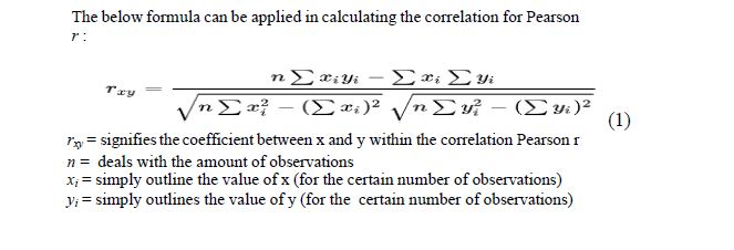
Pearson r correlation
The Pearson r correlation may be viewed as amongst the furthermost broadly applied statistic tool for correlation in order to calculate the gradation of the relationship between linear associated variables. A typical example can be that of a stock market, if one desires to quantify how can two more stocks get to be correlated to one another, Pearson r correlation can s i m p l y b e applied to quantify the notch of the two relationship.
Kendall rank correlation
The correlation of Kendall rank may be deemed as non-parametric test that can be utilized to calculate the strength of dependency within one or two variables. “If one considers models y and z, whereby each model size is n, then one becomes cognizant to the fact that the complete amount of pairings with y z is n(n-1)/2.” [8]. The below 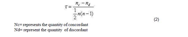 formula can be applied to measure the correlation of Kendall rank ’s value:
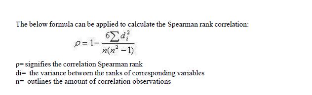
Spearman rank correlation:
Based on (8) the correlation of Spearman rank may be defined as a non-parametric test which can be applied to calculate the gradation of the connotation amongst two or variables. “The tests conducted for Spearman rank doesn’t consist of any assumptions relating to the data distribution and is the suitable correlation analysis whenever the variables are calculated within a scale that is at slightest ordinal variable.
3. Methodology
The experimental findings of our model categorization are discussed in this section.
Experimental Environment
Python and Google Colab were used to implement the experimental findings, and an Intel (R) Core i7 CPU with 8 GB of memory was also used.
Data set
a retroactive sample of men in the Western Cape, South Africa, a heart disease high-risk area. Per case of CHD, there are around two controls. After their CHD occurrence, several of the men who tested positive for CHD had blood pressure lowering therapy and other initiatives to lower
their risk factors. In certain instances, measurements were taken following these procedures. The larger dataset from which these statistics are drawn is given in Rousseauw et al 1983's South African Medical Journal article. Now the dataset are on Kaggle as open-source dataset:
3.1.2 Family history
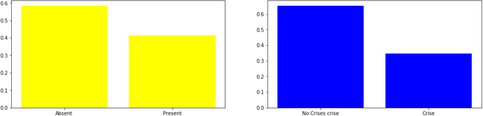
Figure 1. family history of heart diseases
Absent 0.58
Present 0.42
Name: famhist, dtype: float64
0 0.65
1 0.35
Name: chd, dtype: float64
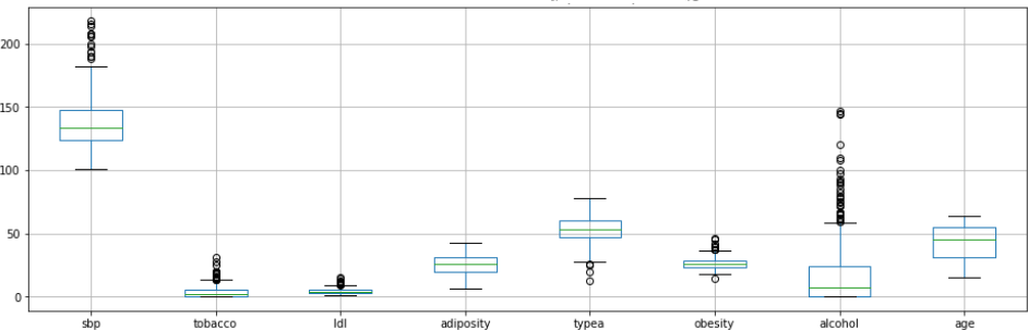
Figure 2: Distribution of the values of potential predictors
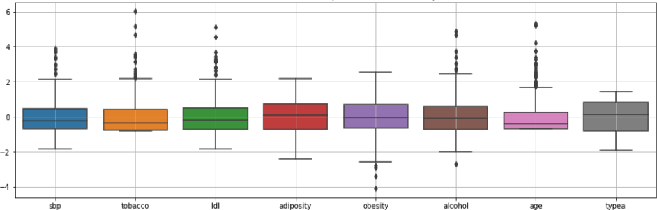
In this instance we have observed a large-Scale difference with various variables. These variables will need to be standardize in order avoid those with greater scales been wrongly having too much weight in the calculations. With Regards to aberrant values, their effect will need to be reduced through methods that are not very sensitive
towards them.
3.2 Dimensionality Reduction
3.2.1 Correlation:
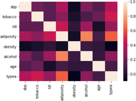
Figure 4: The correlation between various variant
Interpretation
Our observation of the above correlation matrix suggests the following about the coefficient:
• Age has some form of correlation with the consumption of tobacco and level of adiposity.
• There is a strongly correlation between obesity and adiposity.
• Idl is correlated with adiposity.
In summary, the older and obese subjects incline to have additional fats which might be accumulated under the skin.
3.2.2 Bartlett's sphericity test
We conducted the sphericity test and the outcomes value for p was: True. Conclusion of the sphericity test:
Hypothesis: Orthogonality of the variables
Since the p-value is less than the selected threshold, the null hypothesis of orthogonality of variables is rejected.
Therefore: PCA is much relevant within the meaning of this test
We further calculated the Sampling adequacy Kaiser’s measure of (KMO) and the results were kmo: 0.67
Therefore, since the kmo index is between 0.6 and 0.7, a compression relevant index is very possible to be attained. Since some of the values seemed to remain great, we will try a less sensitive approach towards them,
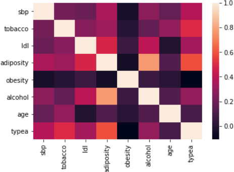
Figure 5: Correlation matrix (Spearman)
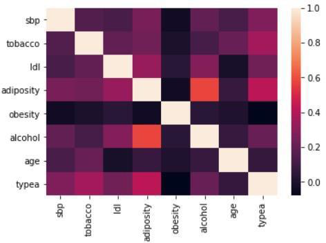
Figure 6: Correlation matrix (Kendall)
A non-parametric PCA based on the Spearman correlation matrix is performed in due to the presence of many atypical values.
Principal Component Analysis (PCA)
PCA is regarded as a model which is applied in covariance structure extended in prepared and established components which carries a declining variance [9]. The inherent data variability is then captured through the features from the linear extraction which are from the novel data sets [10] [11]. The (PCA) Principal components Analysis
is normally founded on correlations are normally gets resolute through the application of a mean centered data.
The data is then gets spit into both training and testing, and the shape for training data was (346, 7) and (116, 7) for testing data
The We calculated the variance ration, variance ration cum sum and variance ration sum
[0.36972103 0.16203157 0.15050121 0.1108632 0. 1 0 1 8 9 0 5 2 ]
[0.36972103 0.5317526 0.68225381 0.793117 0.89500752]
0.8950075163890064
3.3 Predictive analysis
In this section, we went ahead and trained two applied classifiers i.e. random forest (RF) and the Support Vector Machine (SVM). Firstly, on main components, then secondly on the initial data, afterwards we compared their performance by assessing any the contribution in terms of the reduction in size for the decrement of the noise within the predictive model’s construction.
3.3.1 The principal component for Random Forest
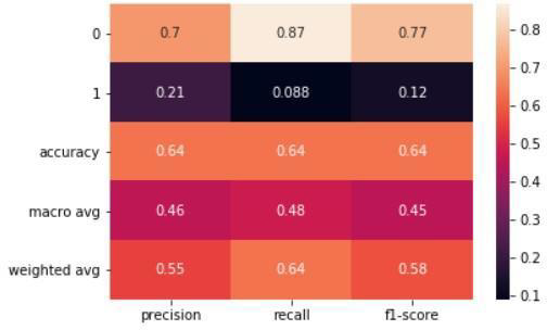
Figure 7: Random Forest Principle component
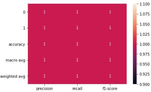
Figure 8: random forest initial Data
3.3.2 The Principal Component for SVM
The principal component for SVM is a technique used in machine learning to reduce the number of features in a dataset by projecting the data onto a new set of orthogonal axes. The goal of this technique is to identify the most important variables in a dataset that capture the majority of the variability in the data. By reducing the number of features, the SVM model can be trained more efficiently and effectively. This results in a more concise and interpretable model that can provide better predictions. In essence, the principal component for SVM is used to maximize the information retention in the reduced dataset while minimizing the loss of information.
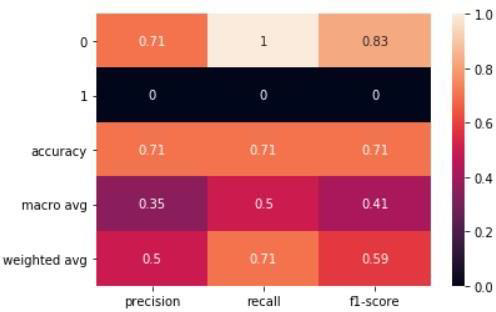
Figure 9. SVM principle component
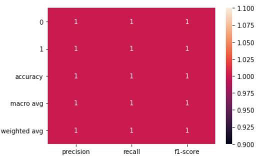
Figure 10: SVM Initial Data
4. Conclusion
In conclusion, it's important to keep in mind that while SVM showed a better accuracy score of 71% compared to Random Forest's score of 61% when PCA was applied, this doesn't always guarantee improved results. Dimensional reduction is just one tool in the machine learning toolkit and there may be other methods and techniques that could lead to even better results. It's essential to consider the limitations of using PCA and to explore other techniques, such as rotating the factorial
axis, to achieve the best outcomes. Additionally, it's important to note that accuracy is not the only evaluation metric to consider. Other metrics, such as precision, recall, F1 score, and receiver operating characteristic (ROC) curve, can provide a more comprehensive understanding of a model's performance. Ultimately, it's crucial to
choose the best model for the task at hand based on a thorough evaluation of multiple metrics and techniques.
References
1. Asha Gowda Karegowda, M.A.Jayaram and A S .Manjunath. Article:Feature Subset Selection using Cascaded GA& CFS: A Filter Approach in Supervised Learning. International Journal of
Computer Applications 23(2):1–10, (June 2011)
2. Bonett, D. G. Meta-analytic interval estimation for bivariate correlations. Psychological Methods, 13(3), 173–181(2008). https://doi.org/10.1037/a0012868
3. Coffman, D. L., Maydeu-Olivares, A., & Arnau, J . Asymptotic distribution free interval estimation: For an intraclass correlation coefficient with applications to longitudinal data. Methodology: European Journal of Research Methods for the Behavioral and Social Sciences, 4(1), 4–9(2008) . https://doi.org/10.1027/1614-2241.4.1.4
4. Shan Xu, Tiangang Zhu, Zhen Zang, Daoxian Wang, Junfeng Hu and Xiaohui Duan et al. “Cardiovascular Risk Prediction Method Based on CFS Subset Evaluation and Random Forest Classification Framework” (2017) IEEE 2nd International Conference on Big Data Analysis
6. J. Padmavathi . A Comparative Study on Logistic Regression Model and PCA-Logistic Regression Model in Medical Diagnosis. International Journal of Engineering and Technology. 2 - 8, 1372-1378. (2012)
7. Kanika Pahwa and Ravinder Kumar et al. “Prediction of Heart Disease Using Hybrid Technique for Selecting Features”, 4th IEEE Uttar Pradesh Section International Conference on Electrical, Computer and Electronics (UPCON). (2017).
8. Swati Shilaskar and Ashok Ghatol. Article: Dimensionality Reduction Techniques for Improved Diagnosis of Heart Disease. International Journal of Computer Applications 61(5):1-8, January (201)3.
9. Jonathon Shlens :A Tutorial on Principal Component Analysis April 22 .Version 3.01, tutorial available at http://www.snl.salk.edu/~shlens/pca.pdf. (2009).
10. R. Zhang, S. Ma, L. Shanahan, J. Munroe, S. Horn, S. Speedie. Automatic methods to extract New York heart association classification from clinical notes IEEE Int Conf Bioinformat Biomed (BIBM) (2017). 10.1109/bibm.2017.8217848
11. G. Parthiban, S.K. Srivatsa: Applying machine learning methods in diagnosing heart disease for diabetic patients Int J Appl Inf Syst, 3 (7) (2012), pp. 25-30, 10.5120/ijais12-450593